•    
  • Machine Learning

    There are two types of machine learning algorithms. Supervised and Unsupervised. Lets look at both

    Supervised Machine Learning

    Provided a set of right answers and a fitted model which is created based on those right answers. Regression Problem is a supervised learning approach to predict a continuous valued output. Classification Problem is where we predict a discrete valued output. Support Vector Machine: Can deal with an infinite number of features

    Unsupervised Machine Learning

    No right answers are given. An example is a clustering algorithm
    -Organize computer clusters, social network analysis, market segmentation, astronomical data analysis etc.
  • Model Representation of a Supervised Learning Algorithm

    Regression Problem -> Predict real valued problem

    Classification Problem -> Predict discrete values

    Learn from data how to predict
    m = mumber of training examples. Together called a training set x = input variables or features y = output variables or target variable (x, y) -> one training example (x(i), y(i)) = ith training example (ie ith row)
    The training set and the learning algorithm together help to create a Hypothesis function (h) or what we refer to above as a model. And this when fed with features of new "experiments" (i.e new measurements about another item that we are trying to predict a class or value of) the model is able to predict the class or value ie the target.

    The Hypothesis Function

    The hypothesis function is represented as
    hθ(x)=θ0 + θ1x This is also referred to as Linear Regression with 1 variable or Univariate Linear Regression

    Here θi's are parameters of the Linear regression with one variable Model. So the problem boils down to "How to choose θ0 and θ1 so that the model from this equation hθ fits the data well.

    Class, Label, Fit, Underfitting and Overfitting

    In classification we are predicting a discrete value of a particular type. For example when we observe the weather conditions and predict if it will "rain" or "not rain" the type is "Whether it will rain". This is the class column. The value that we predict is the label of that column. So we are predicting a class label. Now the class can be of as little as two values (as in this example of rain or not rain) and it is referred to as binary classification or more than that. When multiple values are possible its called multiclass classification problem. Since we are talking about fitting lets define that too. Whenever we find that a model we create using the training set and algorithm is able to make accurate predictions on the new experiments it is a good fit and so we say that the model is able to generalize from the training to the test set. When a model becomes too complex it is called overfitting and when a model is too simple it is called underfitting.

    Training and Creating a Model

    So coming back to our hypothesis function hθ we need to train it so that it is as close as possible in its predictions of the target values to the actual values in the training set. So if hθ(x(i)) are the values predicted by the model and if y(i) are the actual values of the targets in the training data set, we want to caculate the difference between the two and minimze the differnce so that the model fits as closely to the training data set as possible.

    So this now becomes a minimization problem. What are we trying to minimize the difference in the predictions and the actuals. To do this we write a "Cost Function" which is the Sum of the squares of the difference between the predicted and actuals and the whole thing divided by 2 times the number of training values. As we try different values for θ0 and θ1 the value of the cost function changes and we look for the pair of θs so that the value of the cost function is at its least. The value of the cost function traces a plot. Depending on whether we are dealing with only one θ or two we may have a parabola plot or a contour plot. In the case of a parabola we look for that value where the cost function J which describes the slope of the plot approaches zero. In the case of a contour plot we look for those values of θ such that the contour plot described by J is the innermost.
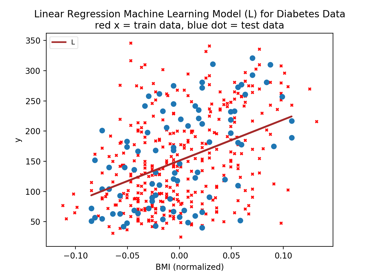
    Linear Regression (Python)


    Image 1: Output image of the Linear Regression Model described below

    Let's first examine the data. The data here is the diabetes dataset. Examining the dataset Bunch object:

    from sklearn import datasets
    To view the raw data
    print dir(datasets.load_diabetes())
    
    • The diabetes dataset consists of 10 physiological variables (age, sex, weight, blood pressure) measure on 442 patients, and an indication of disease progression after one year. You can print out the details with the following command:
      print dir(datasets.load_diabetes())
      Description of the dataset. Here's a link to the paper.This website has more information on this dataset. The dataset in scikit-learn is standarized (zero mean and unit L2 norm). cf http://www.stanford.edu/~hastie/Papers/LARS/ It is the same data as in http://www4.stat.ncsu.edu/~boos/var.select/diabetes.html, but this one (ncsu version) is standarized. (cf 3rd point in http://www.stanford.edu/~hastie/Papers/LARS/) The data in sklearn has therefore lost its physical meaning (age, sex, bmi, blood pressure, ...) Here is a tab separated listing of the data. Here is the description of the load_diabetes function.

      If you dont want to load from sklearn and have the csv of the data set you can import pandas and use the read_csv() function from pandas to import the data into a dataframe.
      Machine Learning Python Code for Linear Regression Model for Diabetes Data Set
      #Application: linear_diabetes.py
      #Author: Vijai Gandikota
      #Date: April 18, 2017
      #Type of Machine Learning Algorithm: Linear Regression
      #Data: Diabetes Dataset
      
      #Import the necessary libraries
      import numpy as np
      import matplotlib.pyplot as plt
      from sklearn import datasets, linear_model
      
      #load the diabetes dataset
      diabetes = datasets.load_diabetes()
      
      #What does the diabetes data set contain (data and target)
      print("\nDiabetes data set has %s" % (dir(diabetes)))
      
      #'sklearn.datasets.base.Bunch'
      print("\nType of the diabetes data structure is %s" % (type(diabetes)))
      
      # I am going to use The 3rd column BMI. This is a normalized data set so we wont see the
      # original data
      diabetes_featuresX = diabetes.data[:, np.newaxis, 3]
      # Assigning the class column
      diabetes_y = diabetes.target
      print("Length of X = %s, Length of y = %s" % (len(diabetes_featuresX), len(diabetes_y)))
      
      # Now we can create the train and test data sets
      # Lets decide what % of the data is test data
      test_percent = 0.2
      print("0.2*len(diabetes_featuresX)= %s " % (int(0.2*len(diabetes_featuresX))))
      # In a list of we do list[:-nn] it will take the last nn records out and assign everything else
      diabetes_featuresX_train = diabetes_featuresX[:int(-0.2*len(diabetes_featuresX))]
      # Now we assign the last 20% of the data to the test set
      diabetes_featuresX_test = diabetes_featuresX[int(-0.2*len(diabetes_featuresX)):]
      
      #Similarly we do the same for the class data
      print("0.2*len(diabetes_y)= %s \n" % (int(0.2*len(diabetes_y))))
      diabetes_y_train = diabetes_y[:int(-0.2*len(diabetes_y))]
      diabetes_y_test = diabetes_y[int(-0.2*len(diabetes_y)):]
      
      #Now I am going to create my linear regression classifier object
      my_LR = linear_model.LinearRegression()
      #Next I'll train the model
      my_LR.fit(diabetes_featuresX_train, diabetes_y_train)
      
      #So we have essential constructed a line. This is a linear equation with coefficients 
      # and variables. So lets print out the coefficients
      print("\nLinear Regression Coefficients = %s" % (my_LR.coef_))
      
      # Next lets test our model and print out the Mean squared error and Variance
      
      # Mean squared error
      # We calculate the mean of the Sum of the squares of the differences between predicted and actual values of y
      mean_squared_error = np.mean(my_LR.predict(diabetes_featuresX_test) - diabetes_y_test) **2
      print("Testing Result: Mean Squared Error = %.3f " % (mean_squared_error))
      
      # Variance
      variance = my_LR.score(diabetes_featuresX_test, diabetes_y_test)
      print("Variance = %.3f " % (variance))
      
      #Now lets plot the train data as little red x's 
      myscatter1=plt.scatter(diabetes_featuresX_train, diabetes_y_train, s=10, color="red", marker="x")
      #Now lets plot the test data as blue dots
      myscatter2=plt.scatter(diabetes_featuresX_test, diabetes_y_test)
      #Now lets print the linear model or the line which shows the predictions of y's from the test set's features
      myplot = plt.plot(diabetes_featuresX_test, my_LR.predict(diabetes_featuresX_test), color="brown", linewidth=2)
      plt.title("Linear Regression Machine Learning Model (L) for Diabetes Data\nred x = train data, blue dot = test data")
      plt.xlabel("BMI (normalized)")
      plt.ylabel("y (normalized)")
      plt.legend(myplot, ('Linear Model'), loc='upper left', framealpha=0.5, prop={'size':'small', 'family':'monospace'})
      plt.show()


      Output
      $ python3.6 linear_diabetes.py 
      
      Diabetes data set has ['data', 'target']
      
      Type of the diabetes data structure is 
      Length of X = 442, Length of y = 442
      0.2*len(diabetes_featuresX)= 88 
      0.2*len(diabetes_y)= 88 
      
      /Library/Frameworks/Python.framework/Versions/3.6/lib/python3.6/site-packages/scipy/linalg/basic.py:1018: RuntimeWarning: internal gelsd driver lwork query error, required iwork dimension not returned. This is likely the result of LAPACK bug 0038, fixed in LAPACK 3.2.2 (released July 21, 2010). Falling back to 'gelss' driver.
        warnings.warn(mesg, RuntimeWarning)
      
      Linear Regression Coefficients = [ 677.53659046]
      Testing Result: Mean Squared Error = 20.215 
      Variance = 0.250 
      ausibm:regression vijai$ python3.6 linear_diabetes.py 
      
      Diabetes data set has ['data', 'target']
      
      Type of the diabetes data structure is 
      Length of X = 442, Length of y = 442
      0.2*len(diabetes_featuresX)= 88 
      0.2*len(diabetes_y)= 88 
      
      /Library/Frameworks/Python.framework/Versions/3.6/lib/python3.6/site-packages/scipy/linalg/basic.py:1018: RuntimeWarning: internal gelsd driver lwork query error, required iwork dimension not returned. This is likely the result of LAPACK bug 0038, fixed in LAPACK 3.2.2 (released July 21, 2010). Falling back to 'gelss' driver.
        warnings.warn(mesg, RuntimeWarning)
      
      Linear Regression Coefficients = [ 677.53659046]
      Testing Result: Mean Squared Error = 20.215 
      Variance = 0.250